

This is the first page for the combined Visual Basic and R approach. Most of this page will use Visual Basic because it is easier to see what it happening. But at the end I will supply R code for a similar analysis. Now I will start right in with an example, because that most easily illustrates the issues that need discussion.
Have you ever thought, when waiting to get someone's parking space, that the driver you are waiting for is taking longer than necessary? Ruback and Juieng (1997) ran a simple study to examine just that question. They hung out in parking lots and recorded the time that it took for a car to leave a parking place. They broke the data down on the basis of whether or not someone in another car was waiting for the space.
Ruback and Juieng observed 200 drivers, but I have reduced that to 20 under each condition, and modified the standard deviation appropriately to maintain the significant difference that they found. I have created what I take to be reasonable data, which means that they are positively skewed, because a driver can safely leave a space only so quickly, but, as we all know, they can sometimes take a very long time. But because the data are skewed, we might feel distinctly uncomfortable using a parametric t test. So we will adopt a randomization test.
The data that I created to reflect the obtained results appear below. The dependent variable is time measured in seconds. (Who would measure such a variable to one hundredth of a second? A guy with a stopwatch that reads in one hundredths of a second.)
No one waiting
36.30 42.07 39.97 39.33 33.76 33.91 39.65 84.92 40.70 39.65
39.48 35.38 75.07 36.46 38.73 33.88 34.39 60.52 53.63 50.62
Someone waiting
49.48 43.30 85.97 46.92 49.18 79.30 47.35 46.52 59.68 42.89
49.29 68.69 41.61 46.81 43.75 46.55 42.33 71.48 78.95 42.06
Now suppose that whether or not someone is waiting for a parking place has absolutely no effect on the driver of the car that is about to vacate that space? Then of the 40 scores that we have here, one of those scores (e.g. 36.30) is equally likely to appear in the No Waiting condition or in the Waiting condition. So, when the null hypothesis is true, any random shuffling of the 40 observations is as likely as any other shuffling to represent the outcome we expect. There certainly is no reason to expect the small numbers to line up under one condition, and the large numbers to line up under the other, although that could happen in some very small percentage of the cases.
There are as many ways that the data could have come out as there are ways of combining the numbers into different groups, and each of those ways is equally likely under the null hypothesis. So one thing that we could theoretically do is to make up all possible arrangements of the data, and then determine whether the arrangement that Ruback and Juieng happened to find is one of the extreme outcomes.
For this example there are 40!/(20!*20!) = 1.3785*1011 combinations, which is a very large number. I don't think that you want to get out your pencil and write down more than 137 billion arrangements--you don't even want your computer to try. But we can get around that by taking a very large number of random samples of the possible arrangements. The other problem is that we need some way of identifying what we mean by an "extreme outcome"--or even what we mean by an "outcome." This leads us to "equivalent statistics."
We use the word "metric" to refer to our unit of measurement. For instance, in this study we measure time in seconds. But we also need some way to measure the difference between groups. In some cases it is pretty clear (here we could record the difference between the means) and in other cases it isn't. Moreover, in some cases several alternative metrics are really equivalent, and in other cases they measure different things.
One way that we could measure an outcome is to take the means of the two groups under any permutation of the data, and declare the difference between the means to be the metric for measuring differences. This is the approach that many authors take, and it is a perfectly legitimate one. At the same time, if we are just rearranging the data that we have, the total of all 40 scores is a constant--it will remain the same for all permutations. So, if we know the total of the first group, we automatically know the total of the second. Thus the mean (or total) of the first group gives us the same information we get from the two means. So we could simply take the mean (or total) of the first group as our metric. It would lead to the same conclusion, and is faster to calculate. I, however, am going to go in the opposite direction. Instead of just taking the difference between the means, I am going to divide that by the standard error of the difference, which will give me a t value. The mean of the first group, the total of the first group, the difference between the means, or the difference standardized by the standard error (i. e., t) will all lead to the same conclusions. The result that gives the most extreme mean of Group 1 will also give the most extreme difference and the most extreme t. I just like t because I am familiar with it, and because it represents the difference relative to the variability of differences. Since I wrote the program, I get to choose. And I chose t.
The following figure shows the results of 5000 shuffles of the data.
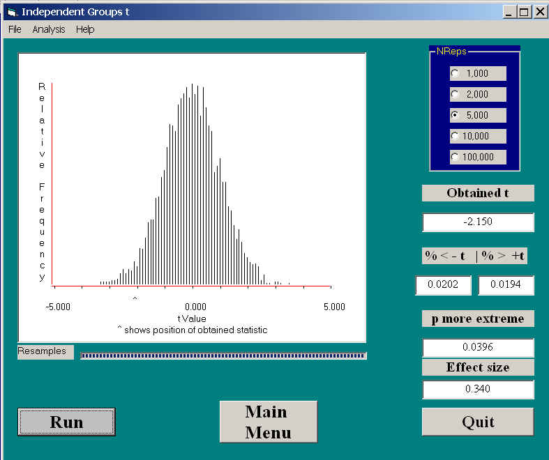
The above figure represents the sampling distribution of the t statistic calculated from 5000 randomizations of the data. Unlike the standard t test, these are not the results of 5000 pairs of samples from a population (or from two identical populations). Unlike the bootstrap procedure, these are not 5000 bootstrapped samples taken, with replacement, from a population consisting of the original observations. These are not samples from any population. They are the results of 5000 random reallocations of the original observations to two groups. Remember, because I am shuffling the data randomly into two groups, the null hypothesis is true. (I might point out here that one of the major differences between randomization tests and bootstrapping is that the former samples without replacement while the latter samples with replacement. But their ultimate purpose is quite different, and the sampling reflects that difference.)
However, the basic question is similar. The question that we are asking is "Would the result that we obtained (here, t = -2.15) be likely to arise if the null hypothesis were true?" The distribution above shows you what t values we would be likely to obtain when the null is true, and you can see that the probability of obtaining a t as extreme as ours is only .0396. At the traditional level of α = .05, we would reject the null hypothesis and conclude that people do, in fact, take a longer time to leave a parking space when someone is sitting there waiting for it.
When we have a traditional Student's t test, one or more extreme scores will likely inflate the mean of that group, and also inflate the within-groups variance. The result is usually, but not always, reflected in a lower value for t, and a lower probability of rejecting the null hypothesis. That is similarly true with the bootstrap, although in that case the resulting distribution would often be expected to be a flatter and broader sampling distribution of t, with again a reduced probability of rejecting the null. But, in a randomization test with two groups, the presence of an outlier often results in a bimodal sampling distribution, depending on which group receives the extreme score in any given randomization.
A nice example can be based on our example of waiting times for parking spaces. Suppose that we have a particularly rude or thoughtless driver who decides that he will let you sit there while he places a call on his cell phone. That call could take a couple of minutes, and would provide an outlier in the data. To simulate this, I replaced the last observation in the Waiting group (42.06 seconds) with an extreme score (242.06 seconds). Because we are permuting the data, rather than sampling, you know that the 242.06 will turn up in every permutation; sometimes in one group, and sometimes in the other. Because it is such a large value, it could cause the sign of the resulting t to swing back and forth between positive and negative, creating an unusual sampling distribution of t.
The result of running the randomization test on the revised data is shown below.
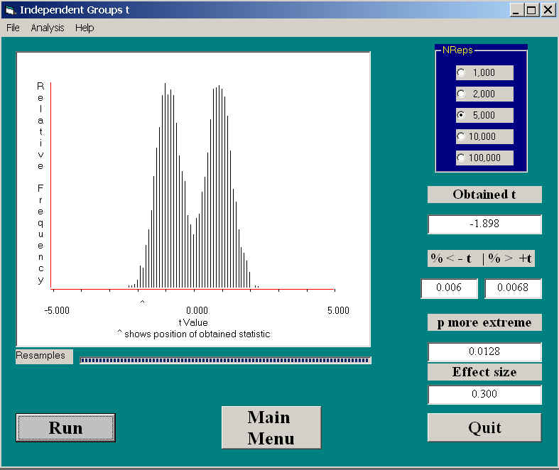
This is certainly not the kind of sampling distribution we normally expect. Aside from the fact that it most closely resembles the hair of Dilbert's manager, it is distinctly different from the distribution Gosset derived. It is symmetrically bimodal, with modes at about +.9 and -1.1. The fact that it is not perfectly symmetric around 0.0 reflects the fact that the distribution, even without the outlier, would be biased in the negative direction due to the generally longer times in the Waiting condition.
Another unusual thing is that the obtained value of t is -1.898, well below the traditional cutoff point for a significant t. Yet, when we look at the results, the actual probability is 0.0128, which is significant. This is a nice illustration that the sampling distribution of t calculated from a randomization test is sometimes quite different from the usual t distribution. Not only is the shape different here, but the critical value is quite a bit smaller.
You should not conclude that the distribution above is a common result of a randomization test on the means of two groups, but it is certainly not unusual. In my limited experience, the sampling distribution is most often similar to the tabled t distribution. However, if you want to see a trimodal sampling distribution, simply make one of the observations in the Non-waiting group equally extreme as well. Again, the data would be completely believable, and a randomization test perfectly defensible, but the results would not look like what we have come to expect with a standard t test.
I like the particular example with which I have been working, because it illustrates a problem that arises with perfectly legitimate data. The first example, where I had no outliers, but where the data were positively skewed in both cases, doesn't present any particular problem. The randomization test simply asks if the data we obtained are a reasonable outcome in an experiment where waiting time is not dependent on the presence or absence of someone waiting for the parking space. In fact, R. A. Fisher (1935) and Pitman (1937) argued that it was in fact the most appropriate test, and that other tests would be legitimate only to the extent that they produced results in line with this test.
For the second example, the randomization test that we looked at was perfectly legitimate. We did not violate any particular assumption, and we can feel very confident in concluding that if waiting time is independent of whether or not someone is waiting for the space, the probability is p = .0128 that these particular observations would fall the way they did. The test itself is just fine. What worries me is whether I should act on these results. The presence of one particular observation made an important difference in the results. I explained why that observation should fall in the Waiting condition, but it seems equally plausible to think of someone who gets in his car, sees no one waiting, and has the good sense to make his cell phone call before he starts driving down the road, rather than while he is driving. But the presence of that observation in the Non-waiting condition would cause the original result to be non-significant. Here the conclusion of the experiment hinges on the result of one observation out of 40, i.e., on 2.5% of the data. That concerns me, not because the statistics are wrong, but because I think that it is poor experimental methodology. This is a case where many mathematically inclined statisticians would talk about trimmed samples, but behavioral scientists rarely use trimmed samples--perhaps out of ignorance.
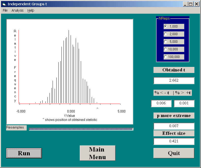
In the discussion of bootstrapping the difference between two medians, I will use a study by Werner et al. (1970) that asked mothers of schizophrenic and normal children to complete a Thematic Apperception Test. The idea was to look for themes of positive parent-child interactions. A randomization test on the two group means is shown below, and here you can see that there were more positive themes in the mothers of normal children. (The small carat below the abscissa represents the location of the obtained statistic.) This difference is significant, at p = .007, with quite a sizeable effect size..
I will now present the code for running a similar analysis in R. There is quite a bit of code here, but it is not particularly difficult to understand. I know that this is going to make for quite a long page, but if you don't like R you can skip right over it.
Although I am not trying to use this page to teach how to code in R, I will show the R code for those who want it. Even if you know nothing about R, I imagine that you can get a sense of what is happening just by looking at the commands. (I hope that you have a copy of R and are able to follow along with the calculations, but, even if you don't, the code should be helpful.) I could have set up separate sections for mean differences and for t, but it is much more efficient to do them together. But I'll first talk about mean differences and then about t.
The following code ran the analyses which follow. The code can be downloaded at TwoSampleTestR.r.
# TwoSampleTestR.r
# Randomization test for difference between two means.
# I will begin using the mean difference as my statistic,
# and then move to using the t statistic for the same purpose.
# When we pool the variances they should give the same result.

NoWaiting <- c(36.30, 42.07, 39.97, 39.33, 33.76, 33.91, 39.65, 84.92, 40.70, 39.65,
39.48, 35.38, 75.07, 36.46, 38.73, 33.88, 34.39, 60.52, 53.63 )
Waiting <- c(49.48, 43.30, 85.97, 46.92, 49.18, 79.30, 47.35, 46.52, 59.68, 42.89,
49.29, 68.69, 41.61, 46.81, 43.75, 46.55, 42.33, 71.48, 78.95)
n1 <- length(NoWaiting)
n2 <- length(Waiting)
N <- n1 + n2
meanNW <- mean(NoWaiting) ; meanW <- mean(Waiting)
diffObt <- (meanW - meanNW)
Combined <- c(NoWaiting, Waiting)     # Combining the samples
    #Now pool the variances
s2p <- (var(NoWaiting)*(n1-1) + var(Waiting)*(n2-1))/(n1 + n2 - 2)
    # Write out the results
cat("The obtained difference between the means is = ",diffObt, '\n')
cat("The pooled variance is = ", s2p, '\n')
cat("Now we will run a standard parametric t test \n")
ttest <- t.test(Waiting, NoWaiting)
cat("The resulting t test on raw data is = ", ttest$statistic, '\n')
print(ttest)
tObt <-  ttest$statistic
nreps <- 5000             # I am using 5000 resamplings of the data
meanDiff <- numeric(nreps)   #Setting up arrays to hold the results
t <- numeric(nreps)
set.seed(1086)        # This means that each run with produce the same results and
                      # agree with the printout that I show.
                      # Remove this line for actual analyses.
for ( i in 1:nreps) {
      data <- sample(Combined, N,  replace = FALSE)
      grp1 <- data[1:n1]
      grp2 <- na.omit(data[n1+1: N])
      meanDiff[i] <- mean(grp1) - mean(grp2)
      test <- t.test(grp1, grp2)
      t[i] <- test$statistic
      }

# Just to demonstrate the equivalence of mean differences and t
cat("The correlation between mean differences and t is = ",'\n')
print(cor(meanDiff, t))
cat('\n')

# Rather than incrementing a counter as I go along, I am counting at the end.
cat("The number of times when the absolute mean differences exceeded diffObt = ",'\n')
absMeanDiff <- abs(meanDiff)
absDiffObt = abs(diffObt)
print(length(absMeanDiff[absMeanDiff >= absDiffObt]))
cat("The number of times when the t values exceeded the obtained t = ",'\n')
abst <- abs(t)
abstObt <- abs(tObt)
print(length(abst[abst >= abstObt]))
cat("The proportion of resamplings when each the mean diff or t exceeded the
obtained value = ",'\n')
print (length(abs(absMeanDiff[absMeanDiff >= absDiffObt]))/nreps)
cat('\n')

par(mfrow = c(2,2))           # Set up graphic window
hist(meanDiff, breaks = 25, ylim = c(0,425))
hist(t, breaks = 50, xlim = c(-5,5), ylim = c(0,425))

#  The following plots the empirical distribution of t from resampling
#     against the actual Student's t distribution on 36 df.
#     Notice the similarity even though the data are badly skewed.
hist(t, freq = FALSE, xlim = c(-5,5), ylim = c(0,.4 ), col = "lightblue",
ylab = "density", xlab = "t", main = "")
par(new = T)
den <- seq(-5, 4.998, .002)
tdens <- dt(den,36)
plot(den, tdens, type = "l", ylim = c(0,.4), xlim = c(-5,5),
  col = "red", ylab = "", xlab = "", main = "Student t and resample t")


# dch   12/3/2013
There is a lot to look at here, but skip the code if you need to. The first set of results tells us that the t test on the difference between means in the actual data was 2.27, which has a probability of only .029. The difference between the two groups means was 10.64 seconds. At the bottom of that section we see that out of 5000 resamples, only 146 times did the mean difference equal or exceed the obtained difference, which represents a proportion of 146/5000 = .0292. (I use absolute differences here because I want a two-tailed test.) This is a small enough percentage to allow us to conclude that the waiting times when someone is waiting for a parking space are significantly longer than when no one is waiting. Of all of the ways that the differences could have come come out, given that having someone waiting does not affect the timing, only about 3% of the time would we expect a difference as great as the one we found. I guess our intuitive feelings are right.
If we had run a standard t test, instead of a resampling test, we would have had a t of 2.27, with an associated probability of .029. Notice how closely, in this particular example, the two probability values agree. That will certainly not always be the case.
Now let's look at the question of what happens if we choose to use the t statistic as our measure of difference instead of the mean difference. We know from the above results that if we had simply run a standard t test on the mean differences, we would have had a very similar result. But we can also see from the following figures that using mean differences or t values as our metric we come to exactly the same result. In fact, in the bottom figure I have gone a step further and asked how the distribution of our t statistics compares to the standard t distribution. I have plotted the t distribution in red on top of the 5000 obtained t values. The distributions are remarkably similar. (Actually, I would have preferred that they be somewhat different to bolster my claim that resampling statistics are the way to go, but it was not to be in this case.)

The above figure represents the sampling distribution of both the mean differences and the t statistic calculated from 5000 randomizations of the data. These are the results of 5000 random reallocations of the original observations to two groups. Remember, because I am shuffling the data randomly into two groups, the null hypothesis is true.
However, the basic question is similar. The question that we are asking is "Would the result that we obtained (here, t = 2.27) be likely to arise if the null hypothesis were true?" The distribution above shows you what t values we would be likely to obtain when the null is true, and you can see that the probability of obtaining a t as extreme as ours is only .0294. At the traditional level of α = .05, we would reject the null hypothesis and conclude that people do, in fact, take a longer time to leave a parking space when someone is sitting there waiting for it.
You may have noticed that I have not referred to any restrictive assumptions behind the test that we have run. One way to understand this is for me to say "I don't care what kinds of populations or parameters lie behind the data, I only want to know how likely is it that, if waiting time is independent of treatment condition, I would get the particular numbers that I have here distributed across groups in the way that they were." Maybe one distribution is very skewed, and the other is completely normal. Perhaps one distribution has a very large variance, and the other has a small one. But my question if simply about the probability that this particular set of data (weird though they may be) would be distributed across groups in the way that they are.
The main reason that we are not concerned about the parent populations, and their parameters, is that we have not randomly sampled from any population. Without random sampling, we don't have a basis to draw inferences about the corresponding parameters. Our interest is quite different from what it is in standard parametric tests, where we at least pretend that we have randomly sampled from populations.
Having said that, I have to go back to the question I have raised elsewhere about the null hypothesis. For the traditional Student's t, the null hypothesis is the μ1 = μ2. We assume that σ12 = σ22 and that the distributions are normal. If we reject the null, we can simply conclude that the population means differ, because there is no other possibility. As Coombs used to say, "You buy data with assumptions." By assuming normality and homogeneity of variance, we buy the conclusion that a significant difference must mean a difference in means.
For this randomization test I have phrased my null hypothesis more loosely. I have taken the null to be "the conditions don't affect the waiting time." I did not state that conditions would not affect the means, or the medians, or the variances, or even the shapes of the distributions. I left that pretty much up in the air.
However, we know from experience that the test is most sensitive to differences in means. In other words, we are more likely to get a significant difference if the two groups' means differ than we are if the two groups' shapes or variances differ. In fact, we usually think of this as a test for location, but that is strictly true only if we are willing to make assumptions about shape and variability.
You may have seen one problem with the TAT example that I just used. Not only have I not randomly sampled participants, but neither have I randomly assigned them to groups. I obviously cannot go out and find 20 students, and then assign 10 of them to a schizophrenic group and 10 to a normal group. But I have said that random assignment lies at the heart of randomization tests, because it justifies our procedure of creating random allocations of the data points.
I would certainly have to plead guilty to violating the condition of random assignment, but I don't think that all is lost. I remain just as confident that if scores were randomly distributed, without regard to group membership, the probability is only .007 that we would have data as extreme as the data we found. In other words,the lack of random assignment does not alter the probability that we have calculated. What it does do is cast doubt on the inferences we can draw from this result. The lack of random assignment prevents me from drawing conclusions about schizophrenia from these data, because it contradicts the rationale for my procedure. Having seen these results, however, I have no doubt that mothers of schizophrenic children produced narratives showing fewer themes of positive parent-child interactions. I have little doubt that if I repeat the study, I would find a similar outcome. But what I cannot do is to draw causal conclusions. It could be that schizophrenic children engage in behavior that leads to poor parent-child interaction. I could be that children who have unresponsive parents are, as a result, more likely to exhibit schizophrenic behavior. My conclusion is valid, but my ability to draw causal inferences from it is not valid.
Wow!!! That's a lot of stuff.
Fisher, R. A. (1935). The design of experiments. Edinburgh:Oliver Boyd
Pitman, E. J. G. (1937). Significance tests which may be applied to samples from any populations. Supplement to The Journal of the Royal Statistical Society, 4, 119-130.
Ruback and Juieng (1997). Journal of Applied Social Psychology, 27, 821-834.
dch:
David C. Howell
University of Vermont
David.Howell@uvm.edu